The RF environment
The RF environment is chaotic. It is complex and diverse. And it is getting worse. Faced with this reality, it is paramount to understand the spectrum and the RF environment to know who is operating, who belongs, and who does not. Geolocation systems serve as crucial tools for identifying, locating, and, when necessary, countering what is taking place within the spectrum.
Geolocation of radio frequency (RF) refers to the process of determining the physical location or source of a specific RF signal or emitter. This process is essential in various fields, from military and defense operations to regulatory spectrum management and interference hunting.
Geolocation techniques are used to pinpoint the origin of a signal—and do so with varying degrees of accuracy based on the method and technology employed.
There are three primary methods CRFS uses to geolocate radio frequency (RF) signals:
- Time Difference of Arrival (TDoA)
- Power of Arrival (PoA)
- Angle of Arrival (AoA)
This article describes how each technique works, illustrates the advantages and disadvantages of each method, and identifies which techniques are best for different types of signals. It also describes the optimal geometry for sensor networks to produce accurate geolocations. Last, it explores new methodologies, including synthetic bearings, and how to understand the elevation of targets over vast areas.
RF geolocation is essential in various fields, from military and defense operations to regulatory spectrum management and interference hunting.
Our dependency on and thirst for bandwidth, driven by our information-based society, presents challenges as the EMS becomes crowded. A crowded spectrum can cause electromagnetic interference, leading to consequences ranging in severity—anything from missing a touchdown in the Super Bowl to a catastrophic military loss.
Our increased usage is causing a dearth of available EMS on a local, national, and international level. Although the EMS is theoretically infinite, there are limits to the useable spectrum available due to a) physical factors constraining operational range and b) the technological capability we have available for its exploitation.
If we wish to continue scaling up our use of the spectrum, it must be used more efficiently and governed in the interest of all citizens. For short-range applications, management can be affected simply by localized spectrum managers, or by using adherence to common sharing protocols such as are standardized for Wi-Fi devices. However, longer-range applications can be more challenging as national bodies must coordinate for smooth and efficient spectrum sharing. The situation becomes more complex near international borders, where authorities from different countries must agree upon and coordinate spectrum use.

Applications of RF geolocation
Military and defense: Locate enemy radars, communication equipment, and other electronic emitters for intelligence purposes and EMCON.
ISR: Pinpoint targets, gather actionable intelligence, and provide real-time situational awareness.
Regulatory spectrum management: Identify sources of interference or unauthorized signal emissions to ensure efficient and compliant spectrum usage.
Law enforcement: Trace illegal or malicious transmissions, such as devices used in criminal activities and illegal radio stations.
Critical infrastructure: Ensure security by continuously monitoring for illicit surveillance devices.
Intelligence agencies: Gather enhanced intelligence by locating threats and conducing counterterrorism and espionage operations.
Industry 4.0: Address the security challenges presented by Industry 4.0, which relies on smart devices connected to wireless networks.
Space launch: Ensure smooth spaceport operations by geolocating any sources of interference.
At a glance: Time Difference of Arrival (TDoA) vs Power on Arrival (PoA) vs Angle of Arrival (AoA)
Time Difference of Arrival (TDoA)
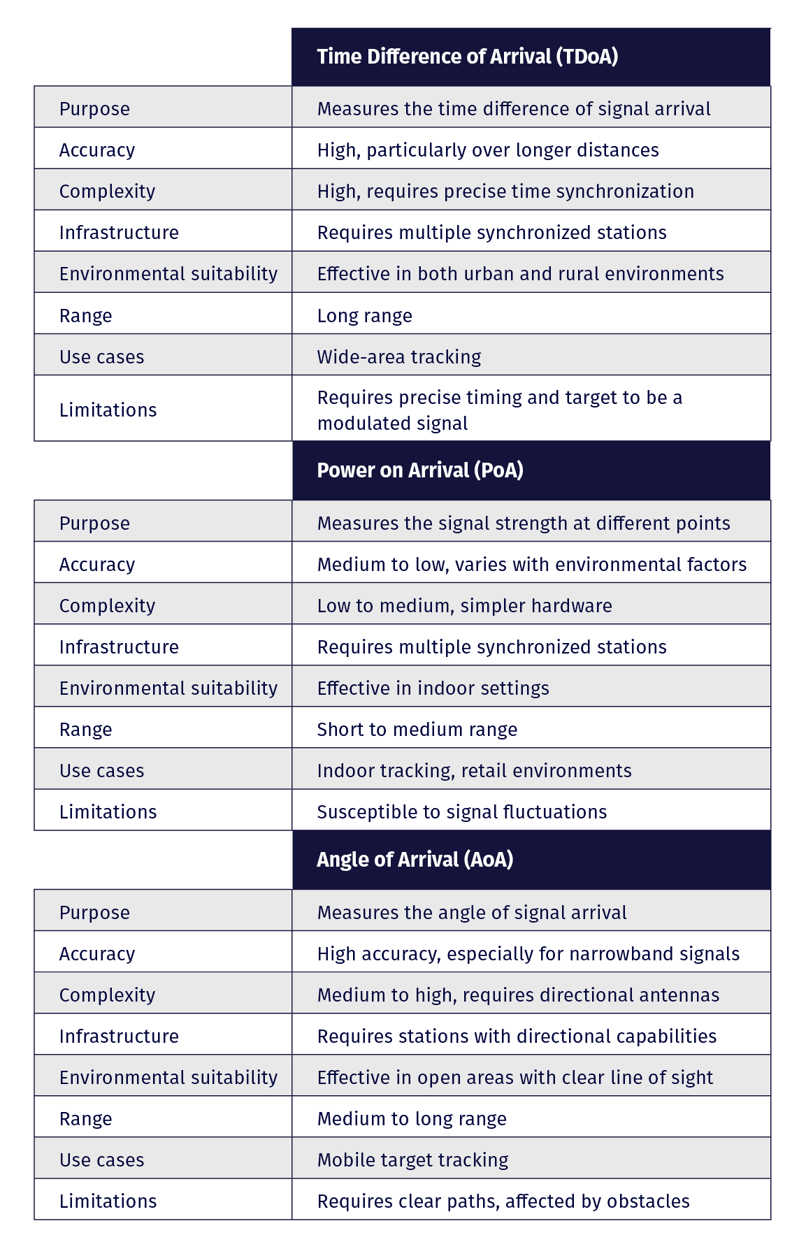
TDoA (also known as multi-lateralization) was developed during the Second World War. The technique compares the time difference of a received RF signal (specifically the I/Q data of the signal) between multiple receivers at one moment in time. As receivers are in different locations, they receive the same signal at different times. Precise calculation of this time difference using spectrum monitoring and geolocation software allows the signals to be geolocated.
Calculating TDoA: To work accurately, TDoA requires an omni antenna and a network of at least three RF receivers, which continuously record RF signals. The data from these signals is sent to a master control computer in real-time, where all signals can be evaluated.
Spectrum monitoring software then overlays the time measurements to ascertain how far (in microseconds or milliseconds) each must be moved until they all line up or correlate. The software also evaluates the quality of how well the signals overlay and uses this information to mitigate multipath and false correlations. The difference between the time measurements represents one correlation point, which the software shows as a single curve (or isochrone) on a map.
Using only two RF receivers, the correlated timing relationship allows a single curve to be formed on a map. Although the signal will be located somewhere along this curve, it is impossible to determine the exact position. However, adding a third sensor allows the software to form a second curve. Based on how the receivers are positioned and the location of the transmitter, a second curve will overlap with the first, and the software will calculate a mathematical latitude-longitude solution.
With this setup, it is possible to compare the timing difference between both sensor pairs, allowing a transmitter to be geolocated in 2D. Given suitable geometry, adding a fourth sensor allows the software to also calculate altitude, using 3D TDoA.
An unlimited number of receivers can be added to a network—on land, in the air, and as fixed or portable deployments. Each sensor will receive a signal at a different time, based on its position with respect to the location of the transmitter. Once the timing relationships are established through correlation, an algorithm uses the known latitude, longitude, and altitude (for 3D purposes) of the receivers to calculate the geolocation of the transmitter.
The RF receiver network: The receiver network should ideally surround the transmitter. If the transmitter moves around inside the network, the sensors can follow the transmission and accurately locate it. However, if the transmitter moves outside the network, geolocating it can become more challenging as the curves meet at very shallow angles. Although the curves will intersect, the shallow angles make it difficult to accurately determine the precise location of the transmitter, which could be located in multiple places where the curves meet.
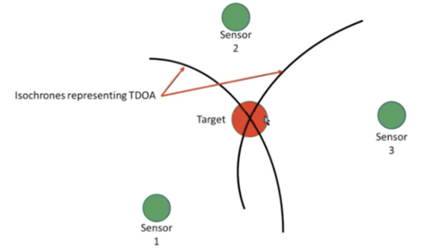
Figure 1: Example of good RF receiver positioning. Two pairs of two receivers create two curves and provide a precise geolocation.
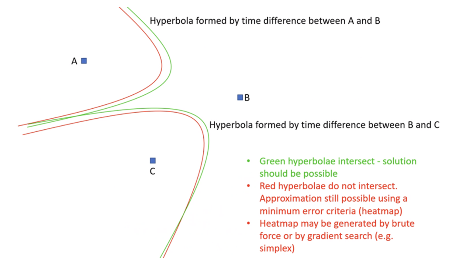
Figure 2: Example of two curves meeting at very shallow angles as the transmitter is located outside the network.
Optimal positioning of RF receivers depends on how many the network comprises. Within a three-sensor network, positioning the sensors in a triangle formation is best practice. With four receivers, optimal results are obtained from a Y-sharp formation, a triangle, plus one receiver located roughly in the middle.
The ideal configuration is multiple receivers placed in a non-symmetrical square formation with at least one sensor inside the box. This will ensure optimal geolocation for both 2D TDoA and 3D TDoA, as there will be no symmetrical intersecting curves, which a symmetrical box shape would produce.
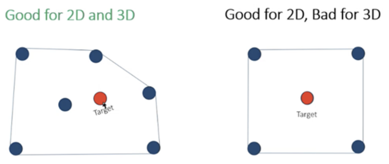 Figure 3: The best results for TDoA and 3D TDoA are produced with a box-shaped network and an internal receiver.
Poor receiver positioning can negatively impact geolocation accuracy. For example, three sensors placed in a straight line can yield ambiguous results: multiple possible geolocations for a signal on the curves between the two pairs of sensors.
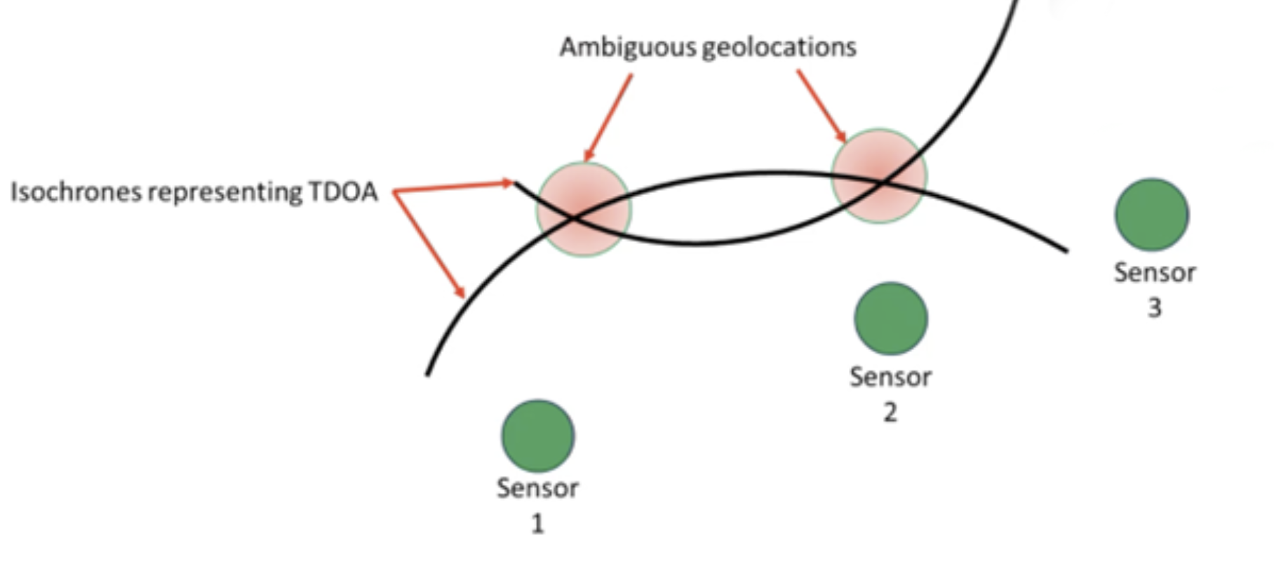
Figure 4: Poor TDoA geometry leads to ambiguous geolocations
The most accurate geolocations will be obtained when the transmitter is located within the RF receiver network; however, it is possible to accurately geolocate a signal at distances up to twice the baseline (the distance between the farthest pair of receivers located in the network). In terms of elevation, the software generally best calculates 3D geolocation (including altitude) when the transmitter’s altitude is within the baseline distance of the receiver network.
Factors affecting the accuracy and performance of TDoA
The accuracy of TDoA geolocation is influenced by modulation bandwidth, which is the range of frequencies used by a signal to transmit information. A transmitter with a modulation bandwidth of 10 MHz could be accurate to 100 meters. However, as the bandwidth decreases, to 1 MHz or 100 kHz, for example, the uncertainty grows significantly, reaching 1500 meters and 5000 meters, respectively.
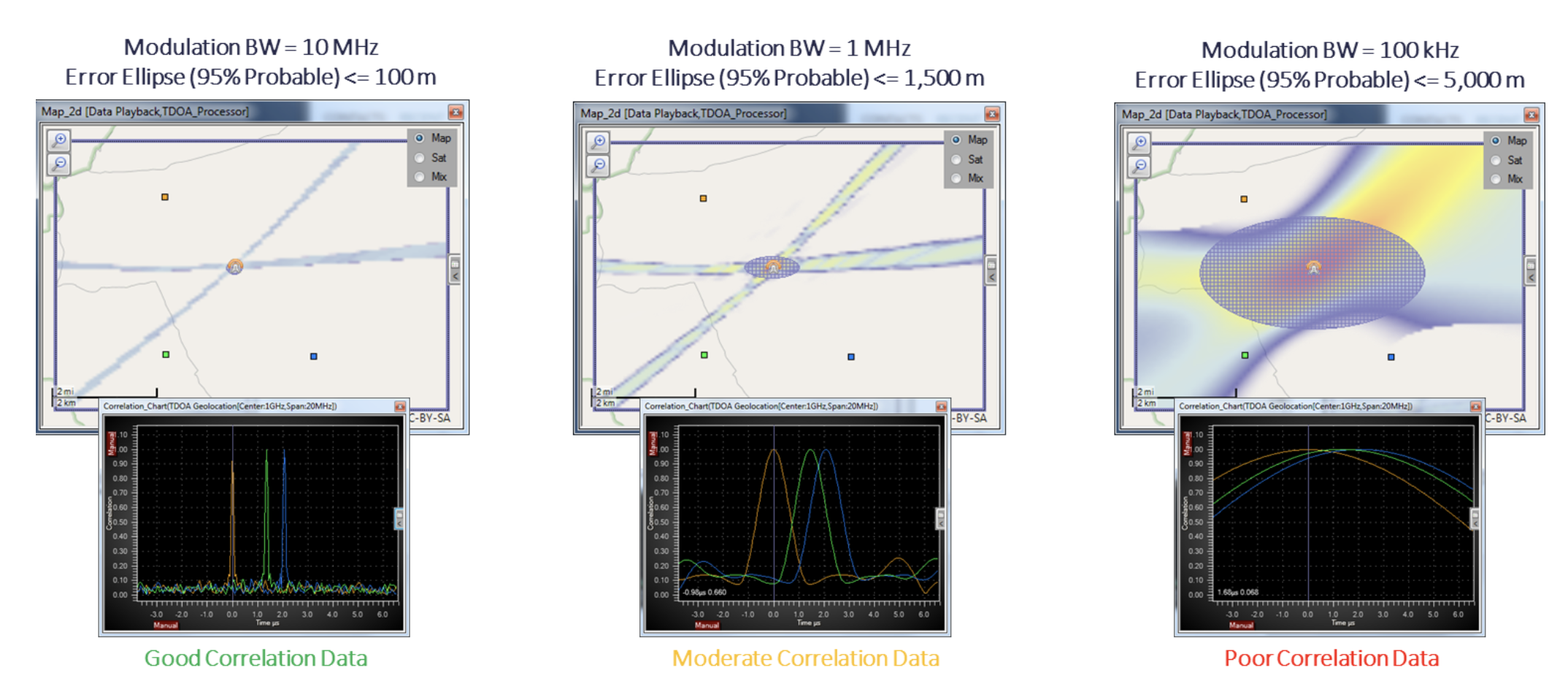
Figure 5: Modulation bandwidth impacting correlation quality
For accurate TDoA, signals must have good correlation properties to measure the precise time difference of a signal arriving at multiple separate receivers. The best type of signals for TDoA are those with a high modulation bandwidth.
Conversely, as modulation bandwidth decreases, less time data is available to correlate, and there are greater timing inaccuracies. Therefore, it becomes more difficult for the software to precisely determine the peaks of the correlation chart.
Although broadband digital modulation yields the most accurate geolocation, systems must be implemented to compensate when signals are not modulated in this way.
Sample-based vs. detector-based TDoA
Sample-based TDoA involves regular, real-time streaming of in-phase and quadrature (I/Q) data (of the signal) back to the control computer, which continuously completes the time correlation between receiver pairs.
This method does not look for any specific type of signal but blindly streams data back to the control computer regardless of signal content. Consequently, this technique can impose heavy demands on the backhaul and may result in the computer wasting time trying to correlate noise.
To counter this, CRFS developed detector-based TDoA, which imposes match filters on the receivers to look for specific signal parameters. For example, detectors can be programmed to evaluate signals with a specific bandwidth over a specified frequency range (i.e., frequency hopping signals), pulsed signals with pre-defined pulse widths (PW), specified pulse repetition intervals (PRI), and more.
If a signal is a fingerprint, signal detectors are fingerprint scanners—they characterize thousands of signals’ frequency, power, and time characteristics in real-time. As the RF receiver is sweeping, the signal detector analyzes and compares each signal against its list of filter criteria looking for matches. Only after a signal matches the filter criteria does the receiver send the I/Q data back to the control computer. In effect, detectors are signal discriminators on a massive scale. When the detector correctly identifies the signal, it initiates the geolocation workflow.
With detector-based TDoA, the receivers retain the I/Q data for a specific amount of time, allowing I/Q data retrieval from the detecting sensor and all other sensors. The correlation engine then takes place, which produces a geolocation. Detector-based TDoA allows for geolocation of frequency hopping signals, whereas sample-based TDoA only correlates against a fixed frequency range. Detector-based TDoA can even search over wide frequency ranges well beyond the RF receivers' instantaneous bandwidth (IBW). This allows correlation and geolocation across wide frequency bands—helping to geolocate frequency-hopping devices such as drones.
More about detectors?
Solutions to identify a signal’s frequency, power, & time characteristics

Locating signals outside the coverage zone using synthetic bearing interference, spoofing, & jamming
At the edge of the coverage zone, curves intersect at shallower angles, making it difficult to ascertain a signal’s position. Therefore, geolocating a transmitter located far outside the network coverage zone can be challenging.
However, a new feature known as synthetic bearing allows the system to form a line of bearing based on the direction the curves are pointing. The bearing indicates that the signal was transmitted somewhere along this line. Software can calculate an approximate range, although range accuracy will deteriorate as the signal moves further away from the receiver network.
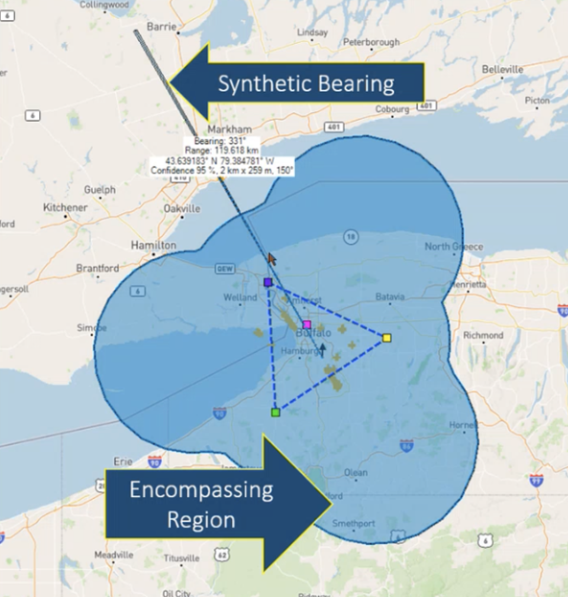
Figure 6: Locating a signal outside the coverage zone using synthetic bearing
Power of Arrival (PoA)
PoA is a geolocation technique that compares the amplitude power (of the signal) received by multiple receivers. It is effective over short distances (typically in an indoor environment). The system analyzes and compares the received power levels to establish a geolocation of a transmitter.
RF receivers in a network are time-synchronized using a CRFS-designed system called SyncLinc, which establishes a precise timing relationship between receivers using either Ethernet or fiber optic cables, resulting in very precise timing accuracies (measured in nanoseconds).
PoA can be used for indoor and outdoor geolocation. Inside a building, sensors are typically installed above ceiling tiles, and can be used to geolocate a specific room in which a transmitter is located. However, a reference sensor should be set up outside a building to distinguish between indoor and outdoor transmissions—crucial for secure facilities.
Calculating PoA
Using an omnidirectional antenna, the farther away the receiver is from the transmitter, the weaker the received signal becomes.
When the signal receiver and the transmitter are close, the software produces a curve with a steep slope and calculates the distance to the transmitter based on RF propagation properties of the signal. By using multiple receivers, these distances can be overlayed on a map to form geolocations.
However, as the transmitter moves further away, the change in power becomes less significant, and the slope becomes shallower. As the slope becomes shallower, PoA becomes less effective. For transmitters located one kilometer away, changes in power become negligible, and the system can no longer effectively calculate the distance.
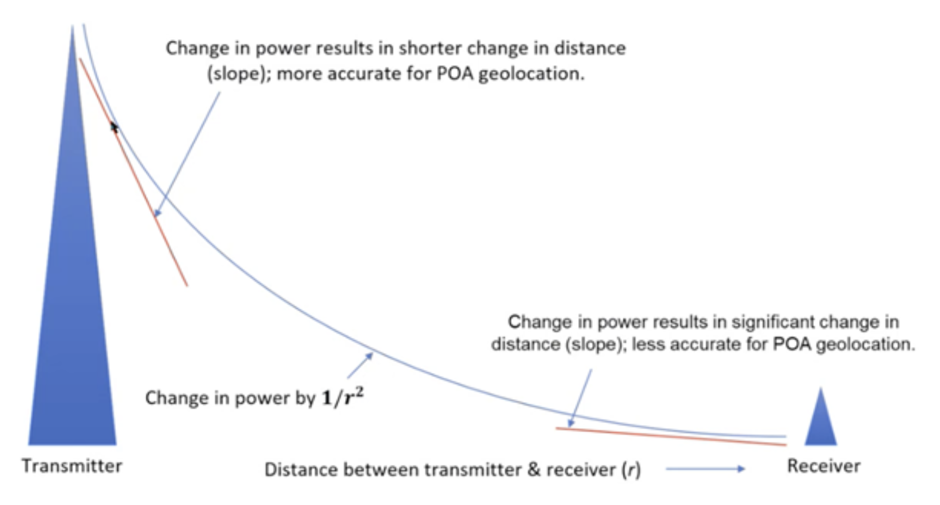
Figure 7: The steep slope of the curve permits accurate geolocation.
Angle of Arrival (AoA)
AoA provides a single line of bearing from a direction finding (DF) Array to a transmitter. The line of bearing can be overlaid on a map or polar chart to indicate where the signal is coming from. The bearing can also be oriented with respect to True North or relative to a mobile vehicle.
AoA looks at the received amplitude of a signal on the faces of six antennas (inside the DF Array) to compare the received amplitude levels. Using the detected signal strength and the known direction of the antenna, the software can establish the direction a signal is coming from with a multi-antenna method. This technique can be used with various fixed and mobile deployment options.
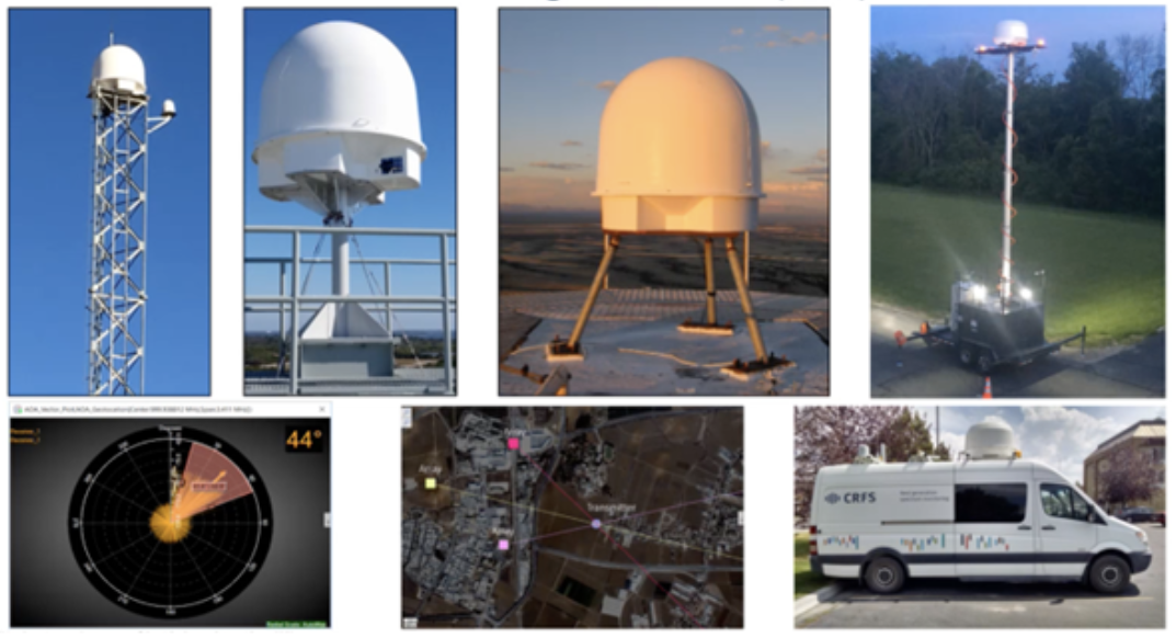
Figure 8: Example of AoA deployments
How does AoA work?
AoA uses a direction-finding Array to geolocate both broadband and narrowband transmitters; however, AoA is the method of choice for narrowband signals.
Each DF Array contains six directional antennas, tuned to listen to one pre-programmed direction. The antennas are situated every 60 degrees in Azimuth, meaning three antennas will always be able to calculate where any one signal is coming from. A power measurement is made at each antenna, and the system then compares the measured power levels to ascertain where the signal is strongest, revealing the transmitter’s direction.
These arrays generally operate up to 18 GHz; however, CRFS has units that operate up to 40 GHz for millimeter-wave applications. CRFS DF arrays can also cover low-band (30 MHz – 300 MHz) DF applications.
AoA is a useful technique for mobile signal hunting. Spectrum managers can drive close to the source of a signal (in a van with an Array) and carry out a geolocation when close.
For even more effective geolocation, using multiple DF arrays will provide multiple lines of bearing, which intersect and show the precise geolocation of a transmitter.
Two high-band DF Array
Each antenna in the Array points in a different direction and picks up the signal from the target of interest on multiple antennas. The system analyzes the signal strength to determine its direction.
If each signal is an arrow pointing in a specific direction, by combining the angle of these arrows, the system gets a clearer idea of where the signal originates. This process helps in tracking the source of a signal, as the antennas can receive the signal, the Array can calculate the line of bearing measurement required for geolocation.
The low-band DF Array
The low-band DF Array has five antennas: four on the outside and one in the center. It determines where a signal is coming from by comparing the signal strength received at each of the outer antennas. The central omnidirectional antenna further refines this by examining signal differences between the outer antennas. Software is then used to combine all these factors to form a line of bearing and establish the direction of the signal.
Every measurement generates a bearing
DF Arrays can track signals of all types, including frequency hopping signals. The CRFS software visualizes these signal directions, using colors to represent either frequency or signal quality. High-quality signals are easier to trace, especially when there is a notable strength difference between antennas on opposite sides of the Array. If the signal strength is almost equal on both sides, it suggests there might be interference or multipath effects, making it harder to determine the exact direction of the original signal.
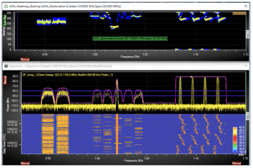
Figure 9: Software showing multiple signals and performing an AoA on a specific frequency domain.
The left side of the figure shows a two-channel frequency hopper, which is generating its own line of bearing as they have their own frequency segments. In the center of the figure is a five-channel frequency hopper with a strong interfering signal in the middle. Generally, when setting up a mission to analyze the signals, the strong interfering signal would dominate the measurement; however, the software can separate signals and analyze them individually, as each generates its own set of frequency segments.
Therefore, it is possible to see the line of bearing from the five-channel frequency hopper and the strong interfering signal. Additionally, tools such as “exclusion zones” can be used to mask out areas within the frequency domain to filter out unwanted signals.
Optimal results from DF Arrays
A single DF Array produces one line of bearing to a transmitter, indicating a signal was transmitted from somewhere along that line. However, to establish distance, a second DF Array should be used from a different location to produce two intersecting lines of bearing, allowing a geolocation to be established. Adding a third DF Array provides an increased degree of accuracy and improved geolocation results, reducing ambiguities and uncertainties.
In terms of positioning RF receivers, placing multiple sensors in a straight line will provide the least accurate results. The system will be more accurate when Arrays surround a target transceiver. Moreover, sensors require line of sight to the transmitting source for optimal geolocation results.
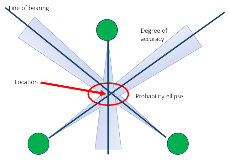
Figure 10: Line of bearing formed from three DF Arrays
While AoA works well on both broadband and narrowband signals, it is the method of choice for narrowband signals. As AoA systems are highly sensitive, it is possible to generate multiple simultaneous lines of bearing.
Conclusion
TDoA, PoA, and AoA make it possible to perform geolocation on most types of RF transmitters. Simultaneously using several of these techniques and comparing the results can improve geolocation accuracy. However, TDoA and PoA are mutually exclusive as the techniques for TDoA require larger baselines, while PoA requires shorter baselines.
Of course, many contributing factors can affect geolocation performance, including transmit frequency, transmit power, modulation type and bandwidth, and antenna height. However, geolocation is only possible when the receiver can “see” the transmitter. Any obstacles obstructing the line of sight will impede geolocation and signal measurement, and if there is no line of sight, geolocation will be impossible. Moreover, elements in the physical environment, such as mirror images from multipath, can also negatively affect geolocation; however, CRFS software uses techniques to mitigate incorrect geolocations based on multipath.
Regardless of the technique, geolocation will only identify the transmitter-radiating elements, which may not necessarily be where the operator is located. In this age of Voice over Internet Protocol (VoIP), the operator could be located far away from the transmitting elements.